Ray Tracer en C++20/23 — du cout à CUDA
Un livre de bout en bout. Tu pars d'un fichier vide, tu finis avec un path tracer parallélisé
capable de produire l'image finale du livre de Peter Shirley — mais entièrement en C++ moderne,
avec concepts, constexpr, std::variant, parallélisme standard, et
un kernel CUDA optionnel.
0.Objectifs et prérequis
0.1 — Ce que tu vas construire
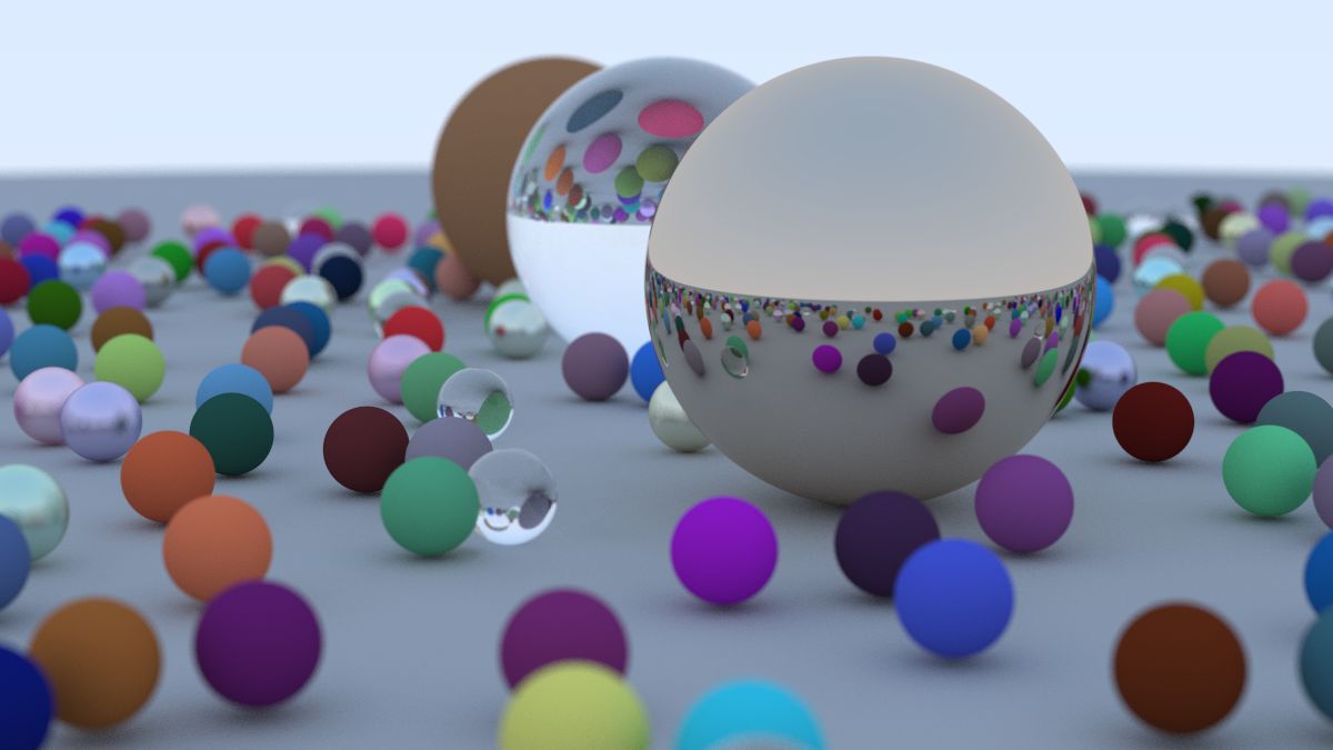
Un path tracer Monte-Carlo : une caméra émet des rayons à travers une grille de pixels, chaque rayon rebondit aléatoirement sur les surfaces, et la couleur du pixel est la moyenne des contributions de centaines d'échantillons. Le résultat tient en une boucle de quelques dizaines de lignes ; tout l'enjeu est de bien typer et ne pas faire d'erreur.
0.2 — Prérequis du cours
- Sections 1 à 8 du cours principal (
index.html) : POO, STL, smart pointers, templates, concepts, ranges, threads. - Compilateur : GCC 13+, Clang 17+, ou MSVC 19.39+.
- CMake 3.28+,
ninjarecommandé. - Optionnel : CUDA 12.4+ pour le chapitre 27.
0.3 — La cible
0.4 — Différences avec le livre original
| Aspect | Livre Shirley | Ce document |
|---|---|---|
| Standard | C++11 « C avec classes » | C++20/23 idiomatique |
| Scalaire | double dur | Template <Scalar T> |
| Polymorphisme | virtual + shared_ptr | std::variant + std::visit |
| Couleur / point / vecteur | Même type vec3 | Trois types distincts (tag dispatch) |
| RNG | Statique (race threads) | thread_local |
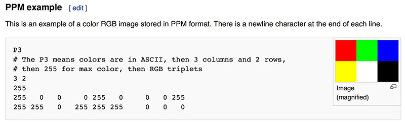
| Sortie | PPM via cout | PNG via stb_image_write |
| Parallélisme | Aucun | std::execution::par_unseq + CUDA optionnel |
| Tests | Aucun | gtest + static_assert |
0.5 — Arborescence du projet
raytracer/
├── CMakeLists.txt
├── third_party/stb_image_write.h
├── include/rt/
│   ├── math.hpp          // vec3, point3, color, dot, cross
│   ├── ray.hpp           // ray<T>
│   ├── interval.hpp      // interval<T>
│   ├── rng.hpp           // RNG thread-local
│   ├── hittable.hpp      // hit_record, concept
│   ├── sphere.hpp
│   ├── material.hpp      // std::variant<Lambertian, Metal, Dielectric>
│   ├── scene.hpp
│   ├── camera.hpp
│   └── image.hpp         // I/O PPM/PNG
├── src/
│   ├── camera.cpp
│   └── render.cpp
├── tests/
│   └── test_math.cpp
└── apps/
└── main.cpp1.Première image — PPM, puis PNG
1.1 — Pourquoi PPM ?
Pour la première image, on n'utilise aucune bibliothèque. Le format PPM (Portable Pixmap) est lisible par tout viewer correct, et son écriture tient en quatre lignes. C'est l'hello world de l'imagerie.
1.2 — Code minimal
On émet une image 256×256 dont le rouge varie horizontalement, le vert verticalement, et le bleu est nul. C'est laid mais ça marche.
// apps/main.cpp — version 1, PPM brut
#include <iostream>

int main() {
    constexpr int W = 256, H = 256;

    std::cout << "P3\n" << W << ' ' << H << "\n255\n";
    for (int y = 0; y < H; ++y) {
        for (int x = 0; x < W; ++x) {
            const int r = static_cast<int>(255.999 * x / (W - 1));
            const int g = static_cast<int>(255.999 * y / (H - 1));
            const int b = 0;
            std::cout << r << ' ' << g << ' ' << b << '\n';
        }
    }
}
Compile, redirige, ouvre :
g++ -std=c++20 -O2 main.cpp -o rt && ./rt > first.ppm
xdg-open first.ppm   # ou: gimp first.ppm, feh first.ppm
1.3 — Critique immédiate
std::coutASCII : ~80 octets par pixel. Pour 1080p ça fait 165 Mo.- Toute autre sortie console casse le fichier.
- Un viewer PPM doit exister sur la machine cible — ce n'est pas garanti.
1.4 — Mieux : PNG via stb_image_write
Une seule dépendance, header-only, domaine public. À garder dès le départ.
// include/rt/image.hpp
#pragma once
#include <span>
#include <cstdint>
#include <filesystem>
#include <stdexcept>
#include <vector>

namespace rt {

struct image_u8 {
    int w, h;
    std::vector<std::uint8_t> rgb;       // taille = w*h*3
};

void write_png(const std::filesystem::path& p, const image_u8& img);

} // rt
// src/image.cpp
#define STB_IMAGE_WRITE_IMPLEMENTATION
#include "stb_image_write.h"
#include "rt/image.hpp"
void rt::write_png(const std::filesystem::path& p, const image_u8& img) {
const int stride = img.w * 3;
if (!stbi_write_png(p.string().c_str(), img.w, img.h, 3, img.rgb.data(), stride))
throw std::runtime_error{"stbi_write_png failed for: " + p.string()};
}std::filesystem::path et pas const char* ?
Pour la même raison qu'on utilise std::string au lieu de char* :
type-safety, encodage Unicode sur Windows, et l'utilisateur peut passer "out.png",
un std::string, ou un path construit programmaticalement.
2.Une barre de progression (au passage)
Quand le rendu va prendre 30 s par image, ne pas avoir de feedback rend le debug pénible.
Une barre minimaliste sur std::cerr (pour ne pas polluer une éventuelle sortie
redirigée) :
// include/rt/progress.hpp
#pragma once
#include <atomic>
#include <chrono>
#include <iostream>

namespace rt {

class progress {
    int total_;
    std::atomic<int> done_{0};
    std::chrono::steady_clock::time_point t0_ = std::chrono::steady_clock::now();
public:
    explicit progress(int total) : total_{total} {}
    void tick(int n = 1) noexcept {
        const int d = done_.fetch_add(n, std::memory_order_relaxed) + n;
        if (d % 256 != 0 && d != total_) return;
        const double pct = 100.0 * d / total_;
        const auto dt = std::chrono::steady_clock::now() - t0_;
        std::cerr << "\r" << int(pct) << "% (" << d << "/" << total_
                  << ") "
                  << std::chrono::duration_cast<std::chrono::seconds>(dt).count() << "s   ";
        if (d == total_) std::cerr << "\n";
    }
};

}memory_order_relaxed ? Le compteur n'a aucune dépendance avec
d'autres données mémoire. On veut juste l'incrémenter atomiquement. relaxed évite la
barrière mémoire, accélérant le hot path. Cours 7.4.
3.vec3<T> — algèbre 3D templatisée
3.1 — Cahier des charges
Notre vec3 doit être :
- Paramétré par le type scalaire (
floaten prod,doubleen debug). constexprpartout où c'est possible.- Trivialement copiable : pas d'allocation, pas de pointeur, juste 3 flottants.
- Comparable (
operator<=>) pour les tests.
3.2 — Implémentation
// include/rt/math.hpp
#pragma once
#include <array>
#include <cmath>
#include <concepts>
#include <limits>
#include <ostream>

namespace rt {

template <typename T>
concept Scalar = std::floating_point<T>;

template <Scalar T>
class vec3 {
    std::array<T, 3> e_{};
public:
    constexpr vec3() noexcept = default;
    constexpr vec3(T x, T y, T z) noexcept : e_{x, y, z} {}

    [[nodiscard]] constexpr T x() const noexcept { return e_[0]; }
    [[nodiscard]] constexpr T y() const noexcept { return e_[1]; }
    [[nodiscard]] constexpr T z() const noexcept { return e_[2]; }
    [[nodiscard]] constexpr T operator[](std::size_t i) const noexcept { return e_[i]; }

    [[nodiscard]] constexpr T length_squared() const noexcept {
        return e_[0]*e_[0] + e_[1]*e_[1] + e_[2]*e_[2];
    }
    [[nodiscard]] T length() const noexcept { return std::sqrt(length_squared()); }

    [[nodiscard]] constexpr bool near_zero() const noexcept {
        constexpr T eps = T(1e-8);
        return std::fabs(e_[0]) < eps && std::fabs(e_[1]) < eps && std::fabs(e_[2]) < eps;
    }

    constexpr vec3& operator+=(vec3 v) noexcept { e_[0]+=v.e_[0]; e_[1]+=v.e_[1]; e_[2]+=v.e_[2]; return *this; }
    constexpr vec3& operator*=(T s)    noexcept { e_[0]*=s; e_[1]*=s; e_[2]*=s; return *this; }
    constexpr vec3& operator/=(T s)    noexcept { return *this *= T(1) / s; }

    [[nodiscard]] constexpr vec3 operator-() const noexcept { return {-e_[0], -e_[1], -e_[2]}; }

    friend constexpr auto operator<=>(vec3, vec3) = default;
};

// Opérateurs binaires libres : pas amis, pas membres → ADL propre
template <Scalar T> [[nodiscard]] constexpr vec3<T> operator+(vec3<T> a, vec3<T> b) noexcept { return {a.x()+b.x(), a.y()+b.y(), a.z()+b.z()}; }
template <Scalar T> [[nodiscard]] constexpr vec3<T> operator-(vec3<T> a, vec3<T> b) noexcept { return {a.x()-b.x(), a.y()-b.y(), a.z()-b.z()}; }
template <Scalar T> [[nodiscard]] constexpr vec3<T> operator*(vec3<T> a, vec3<T> b) noexcept { return {a.x()*b.x(), a.y()*b.y(), a.z()*b.z()}; } // hadamard, utile pour color
template <Scalar T> [[nodiscard]] constexpr vec3<T> operator*(T s, vec3<T> v)        noexcept { return {s*v.x(), s*v.y(), s*v.z()}; }
template <Scalar T> [[nodiscard]] constexpr vec3<T> operator*(vec3<T> v, T s)        noexcept { return s * v; }
template <Scalar T> [[nodiscard]] constexpr vec3<T> operator/(vec3<T> v, T s)        noexcept { return v * (T(1)/s); }

template <Scalar T> [[nodiscard]] constexpr T dot(vec3<T> a, vec3<T> b) noexcept { return a.x()*b.x() + a.y()*b.y() + a.z()*b.z(); }
template <Scalar T> [[nodiscard]] constexpr vec3<T> cross(vec3<T> a, vec3<T> b) noexcept {
    return { a.y()*b.z() - a.z()*b.y(),
             a.z()*b.x() - a.x()*b.z(),
             a.x()*b.y() - a.y()*b.x() };
}
template <Scalar T> [[nodiscard]] vec3<T> unit(vec3<T> v) noexcept { return v / v.length(); }

// Constantes mathématiques (cours 5.6 : inline constexpr garantit une seule définition)
template <Scalar T> inline constexpr T pi_v  = T(3.141592653589793238L);
template <Scalar T> inline constexpr T inf_v = std::numeric_limits<T>::infinity();

template <Scalar T>
[[nodiscard]] constexpr T deg_to_rad(T d) noexcept { return d * pi_v<T> / T(180); }

} // rt
3.3 — Tests à la compilation
static_assert(rt::vec3<float>{1,2,3}.length_squared() == 14.0f);
static_assert(rt::dot(rt::vec3<float>{1,0,0}, rt::vec3<float>{0,1,0}) == 0.0f);
static_assert(rt::cross(rt::vec3<float>{1,0,0}, rt::vec3<float>{0,1,0}).z() == 1.0f);- Test math gratuit : si
dotest cassé, le code ne compile pas. - Compatible CUDA via
RT_HDà ajouter au chapitre 27. - Pas une seule allocation. Tout passe par registres.
4.color<T> — typage fort à coût nul
4.1 — Le piège du livre
Dans le livre original, on lit :
using point3 = vec3;
using color  = vec3;
Trois noms, un seul type. Conséquence directe : color c = position * scale compile,
et personne ne s'aperçoit que tu viens de multiplier une couleur par un mètre.
4.2 — Solution : tag dispatch
Un type fantôme par catégorie, paramétrant le même layout mémoire. Coût runtime : zéro (le compilateur supprime le tag en optimisation). Bénéfice : trois types distincts.
// dans rt/math.hpp, après vec3
namespace rt {

template <Scalar T>
class point3 {
    vec3<T> v_{};
public:
    constexpr point3() noexcept = default;
    constexpr point3(T x, T y, T z) noexcept : v_{x,y,z} {}
    [[nodiscard]] constexpr T x() const noexcept { return v_.x(); }
    [[nodiscard]] constexpr T y() const noexcept { return v_.y(); }
    [[nodiscard]] constexpr T z() const noexcept { return v_.z(); }
    [[nodiscard]] constexpr explicit operator vec3<T>() const noexcept { return v_; }
    friend constexpr auto operator<=>(point3, point3) = default;
};

// point + vec = point ; point - point = vec
template <Scalar T>
[[nodiscard]] constexpr point3<T> operator+(point3<T> p, vec3<T> v) noexcept {
    return {p.x()+v.x(), p.y()+v.y(), p.z()+v.z()};
}
template <Scalar T>
[[nodiscard]] constexpr vec3<T> operator-(point3<T> a, point3<T> b) noexcept {
    return {a.x()-b.x(), a.y()-b.y(), a.z()-b.z()};
}

// color est un vec3, mais distinct via tag
struct color_tag {};
template <Scalar T>
class color {
    vec3<T> v_{};
public:
    constexpr color() noexcept = default;
    constexpr color(T r, T g, T b) noexcept : v_{r,g,b} {}
    [[nodiscard]] constexpr T r() const noexcept { return v_.x(); }
    [[nodiscard]] constexpr T g() const noexcept { return v_.y(); }
    [[nodiscard]] constexpr T b() const noexcept { return v_.z(); }

    constexpr color& operator+=(color c) noexcept { v_ += c.v_; return *this; }
    constexpr color& operator*=(T s)    noexcept { v_ *= s;   return *this; }
};

template <Scalar T> [[nodiscard]] constexpr color<T> operator+(color<T> a, color<T> b) noexcept { return {a.r()+b.r(), a.g()+b.g(), a.b()+b.b()}; }
template <Scalar T> [[nodiscard]] constexpr color<T> operator*(color<T> a, color<T> b) noexcept { return {a.r()*b.r(), a.g()*b.g(), a.b()*b.b()}; } // atténuation
template <Scalar T> [[nodiscard]] constexpr color<T> operator*(T s, color<T> c)         noexcept { return {s*c.r(), s*c.g(), s*c.b()}; }
template <Scalar T> [[nodiscard]] constexpr color<T> operator*(color<T> c, T s)         noexcept { return s * c; }

}
4.3 — Conversion couleur → octets
namespace rt {

template <Scalar T>
[[nodiscard]] std::uint8_t to_byte(T x) noexcept {
    // clamp [0,1] puis quantize
    x = std::clamp(x, T(0), T(0.999));
    return static_cast<std::uint8_t>(256 * x);
}

template <Scalar T>
void write_pixel(image_u8& img, int x, int y, color<T> c) {
    const int i = (y * img.w + x) * 3;
    img.rgb[i+0] = to_byte(c.r());
    img.rgb[i+1] = to_byte(c.g());
    img.rgb[i+2] = to_byte(c.b());
}

}5.ray<T> — un point et une direction
Un rayon est paramétrique : P(t) = O + t·D. Origine, direction, et un scalaire
pour parcourir.
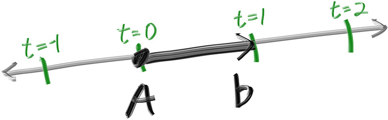
P(t) parcourt la droite quand t varie.
Source : raytracing.github.io// include/rt/ray.hpp
#pragma once
#include "rt/math.hpp"
namespace rt {
template <Scalar T>
class ray {
point3<T> orig_{};
vec3<T> dir_{};
public:
constexpr ray() noexcept = default;
constexpr ray(point3<T> o, vec3<T> d) noexcept : orig_{o}, dir_{d} {}
[[nodiscard]] constexpr point3<T> origin() const noexcept { return orig_; }
[[nodiscard]] constexpr vec3<T> direction() const noexcept { return dir_; }
[[nodiscard]] constexpr point3<T> at(T t) const noexcept { return orig_ + t * dir_; }
};
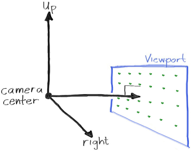
}6.Caméra primitive et fond dégradé
6.1 — Géométrie
On place la caméra à l'origine, on définit un viewport (la fenêtre virtuelle dans laquelle on tire les rayons), et on émet un rayon par pixel. Pas de profondeur de champ, pas de FOV configurable encore — on ajoutera ça aux chapitres 22–23.
z = -focal_length.
Source : raytracing.github.iodelta_u et delta_v.
Source : raytracing.github.io6.2 — Fond : dégradé bleu / blanc
Quand un rayon ne touche rien, on retourne une couleur dépendant de sa direction Y normalisée. C'est purement esthétique — on simule un ciel.
template <Scalar T>
[[nodiscard]] color<T> sky(const ray<T>& r) noexcept {
    const auto u = unit(r.direction());
    const T a = T(0.5) * (u.y() + T(1));
    return (T(1) - a) * color<T>{1,1,1} + a * color<T>{0.5, 0.7, 1.0};
}
6.3 — Boucle de rendu naïve
int main() {
    using F = float;
    constexpr F aspect = 16.0f / 9.0f;
    constexpr int W = 400;
    constexpr int H = static_cast<int>(W / aspect);

    constexpr F focal = 1.0f;
    constexpr F vh = 2.0f;
    constexpr F vw = vh * static_cast<F>(W) / H;

    const rt::point3<F> cam{0,0,0};
    const rt::vec3<F>   du{vw, 0, 0}, dv{0, -vh, 0};
    const rt::vec3<F>   pixel_du = du / static_cast<F>(W);
    const rt::vec3<F>   pixel_dv = dv / static_cast<F>(H);
    const rt::point3<F> vp_top_left = cam + rt::vec3<F>{0,0,-focal} - du/2.0f - dv/2.0f;
    const rt::point3<F> pixel00 = vp_top_left + 0.5f * (pixel_du + pixel_dv);

    rt::image_u8 img{W, H, std::vector<std::uint8_t>(W * H * 3)};
    for (int y = 0; y < H; ++y)
        for (int x = 0; x < W; ++x) {
            const auto p = pixel00 + static_cast<F>(x) * pixel_du + static_cast<F>(y) * pixel_dv;
            const rt::ray<F> r{cam, p - cam};
            rt::write_pixel(img, x, y, rt::sky(r));
        }
    rt::write_png("out.png", img);
}
main. C'est OK
pour ce chapitre, mais on va l'extraire dans une classe au chapitre 14.
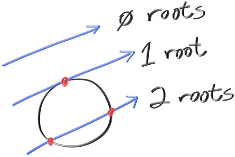
7.Une sphère
Une sphère de centre C et rayon r satisfait
(P − C)·(P − C) = r². En substituant P = O + tD, on obtient une équation
quadratique en t. Le discriminant détermine le nombre de solutions.
7.1 — Première version : booléen seul
template <Scalar T>
[[nodiscard]] bool hits_sphere(point3<T> center, T radius, const ray<T>& r) noexcept {
    const auto oc = r.origin() - center;     // vec3 (point - point = vec)
    const T a = dot(r.direction(), r.direction());
    const T b = T(2) * dot(oc, r.direction());
    const T c = dot(oc, oc) - radius * radius;
    return (b * b - T(4) * a * c) >= T(0);
}
On peint la sphère en rouge et on regarde :
if (hits_sphere<F>({0,0,-1}, 0.5f, r)) return rt::color<F>{1,0,0};
t < 0 (sphère derrière
la caméra). Si tu déplaces la caméra de l'autre côté, la sphère reste rouge. À corriger avec un
intervalle, chapitre 13.
8.Intersection qui retourne le t
On va vouloir colorier la sphère en fonction de la normale. Pour ça, il nous faut le point
d'intersection, donc le t. On retourne std::optional<T> :
template <Scalar T>
[[nodiscard]] std::optional<T>
hits_sphere(point3<T> center, T radius, const ray<T>& r) noexcept {
    const auto oc = r.origin() - center;
    // Astuce : on remplace b par h = b/2 → moins de multiplications
    const T a    = dot(r.direction(), r.direction());
    const T h    = dot(oc, r.direction());
    const T c    = dot(oc, oc) - radius * radius;
    const T disc = h * h - a * c;
    if (disc < T(0)) return std::nullopt;
    return (-h - std::sqrt(disc)) / a;     // racine la plus proche
}std::optional et pas un sentinelle (-1.0 par exemple) ?
Parce que le compilateur t'oblige à gérer le nullopt avec
if (auto t = hits_sphere(...)), et tu ne peux pas oublier. Aucun équivalent C-style
n'est aussi sûr.
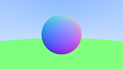
9.Normales de surface
Sur une sphère, la normale au point P est (P − C) / r. On colorie en
visualisant la normale comme un RGB pour voir qu'elle est correcte.
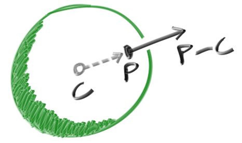
P − C, normalisée par r.
Source : raytracing.github.iotemplate <Scalar T>
[[nodiscard]] color<T> ray_color(const ray<T>& r) noexcept {
if (auto t = hits_sphere<T>({0,0,-1}, 0.5, r)) {
const auto n = unit(r.at(*t) - point3<T>{0,0,-1});
// remap [-1,1] → [0,1] pour visualiser
return 0.5 * color<T>{n.x() + 1, n.y() + 1, n.z() + 1};
}
return sky(r);
}
10.hittable : virtual ou variant ? Le grand débat
Maintenant qu'on veut plusieurs sphères (et plus tard d'autres primitives), on a besoin d'une abstraction. Le livre choisit l'héritage virtuel. C'est le bon réflexe en 2003. En 2026, on a un meilleur outil pour ce cas précis.
10.1 — Le choix par défaut du livre (qu'on n'utilisera pas)
// Approche du livre — pédagogiquement claire mais pas optimale
class hittable {
public:
    virtual ~hittable() = default;
    virtual bool hit(const ray&, interval, hit_record&) const = 0;
};
class sphere : public hittable { ... };
// Stockage : std::vector<std::shared_ptr<hittable>>
10.2 — Pourquoi ce n'est pas le bon choix ici
| Critère | virtual + shared_ptr | std::variant + std::visit |
|---|---|---|
| Coût dispatch (chaud) | vtable + cache miss : ~5 ns | switch sur index : ~1 ns |
| Allocation | 1 alloc/objet (heap fragmenté) | 0 alloc (stocké inline) |
| Compteur de réf | Atomique → contention threads | Aucun |
| Extensibilité runtime (plugin) | Oui | Non — recompilation |
| Compatible CUDA | Non | Oui (libcu++) |
| Set fermé connu à compile-time | Cache un fait certain | L'exprime explicitement |
Ici, l'ensemble des primitives est connu : sphère, plan, triangle. Pas de plugin
utilisateur. C'est exactement le cas d'usage de std::variant.
10.3 — hit_record et concept
// include/rt/hittable.hpp
#pragma once
#include "rt/math.hpp"
#include "rt/ray.hpp"
#include "rt/interval.hpp"
#include <cstdint>
#include <optional>

namespace rt {

template <Scalar T>
struct hit_record {
    point3<T>     p;
    vec3<T>       normal;       // toujours dirigée contre le rayon
    T              t;
    bool           front_face;
    std::uint32_t material_id;
};

// Concept : tout ce qui sait répondre à hit() est un Hittable
template <typename H, typename T>
concept Hittable = Scalar<T> && requires(const H h, ray<T> r, interval<T> iv) {
    { h.hit(r, iv) } -> std::same_as<std::optional<hit_record<T>>>;
};

}hit() avec la bonne signature, mais ne le vérifie pas
intrinsèquement. Le concept l'impose et donne des erreurs de compilation lisibles.
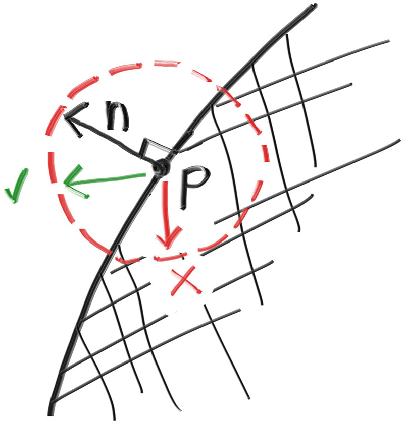
11.Front face / back face
Quand un rayon traverse une surface (verre par exemple), on doit savoir s'il entre ou
sort. La convention adoptée : la normale stockée dans hit_record pointe
toujours contre le rayon (sortante de la surface vue par le rayon).
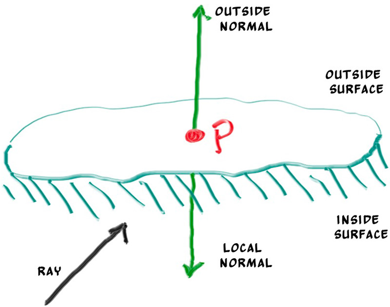
front_face.
Source : raytracing.github.iotemplate <Scalar T>
[[nodiscard]] constexpr hit_record<T>
make_hit(T t, point3<T> p, vec3<T> outward, const ray<T>& r, std::uint32_t mat) noexcept {
const bool ff = dot(r.direction(), outward) < T(0);
return {p, ff ? outward : -outward, t, ff, mat};
}set_face_normal qui mute
hit_record. Notre version est une fonction libre qui retourne par valeur — moins
d'invariants à mémoriser, copies optimisées (RVO).
12.Scène : vector de primitives via variant
12.1 — La sphère, version finale
// include/rt/sphere.hpp
#pragma once
#include "rt/hittable.hpp"
#include <stdexcept>

namespace rt {

template <Scalar T>
class sphere {
    point3<T>     center_;
    T              radius_;
    std::uint32_t mat_id_;
public:
    constexpr sphere(point3<T> c, T r, std::uint32_t m)
        : center_{c}, radius_{r}, mat_id_{m}
    {
        if (r <= T(0)) throw std::invalid_argument{"sphere: radius > 0"};
    }

    [[nodiscard]] std::optional<hit_record<T>>
    hit(const ray<T>& r, interval<T> iv) const noexcept {
        const auto oc = r.origin() - center_;
        const T a    = dot(r.direction(), r.direction());
        const T h    = dot(oc, r.direction());
        const T c    = dot(oc, oc) - radius_ * radius_;
        const T disc = h * h - a * c;
        if (disc < T(0)) return std::nullopt;

        const T sd = std::sqrt(disc);
        T root = (-h - sd) / a;
        if (!iv.surrounds(root)) {
            root = (-h + sd) / a;
            if (!iv.surrounds(root)) return std::nullopt;
        }
        const auto p = r.at(root);
        const auto outward = (p - center_) / radius_;
        return make_hit(root, p, outward, r, mat_id_);
    }
};

static_assert(Hittable<sphere<float>, float>);

}
12.2 — La scène
// include/rt/scene.hpp
#pragma once
#include "rt/sphere.hpp"
#include "rt/material.hpp"
#include <variant>
#include <vector>

namespace rt {

template <Scalar T>
using primitive = std::variant<sphere<T>/*, plane<T>, triangle<T>...*/>;

template <Scalar T>
[[nodiscard]] std::optional<hit_record<T>>
hit(const primitive<T>& p, const ray<T>& r, interval<T> iv) {
    return std::visit([&](const auto& obj) { return obj.hit(r, iv); }, p);
}

template <Scalar T>
class scene {
    std::vector<primitive<T>> prims_;
    std::vector<material<T>>  mats_;
public:
    std::uint32_t add_material(material<T> m) {
        mats_.push_back(m);
        return static_cast<std::uint32_t>(mats_.size() - 1);
    }
    void add(primitive<T> p) { prims_.push_back(p); }

    [[nodiscard]] const material<T>& material_of(std::uint32_t id) const noexcept { return mats_[id]; }

    [[nodiscard]] std::optional<hit_record<T>>
    hit_world(const ray<T>& r, interval<T> iv) const {
        std::optional<hit_record<T>> closest;
        T t_max = iv.max();
        for (const auto& p : prims_) {
            if (auto rec = rt::hit(p, r, {iv.min(), t_max})) {
                t_max  = rec->t;
                closest = rec;
            }
        }
        return closest;
    }
};

}
13.interval<T> — borner les t
À chaque test d'intersection on a besoin d'un domaine valide : t > 0 (devant la
caméra) et t < t_closest (plus proche que la meilleure trouvée). Une mini-classe
rend l'API plus claire qu'une paire de scalaires.
// include/rt/interval.hpp
#pragma once
#include "rt/math.hpp"

namespace rt {

template <Scalar T>
class interval {
    T mn_, mx_;
public:
    constexpr interval() noexcept : mn_{+inf_v<T>}, mx_{-inf_v<T>} {}
    constexpr interval(T a, T b) noexcept : mn_{a}, mx_{b} {}

    [[nodiscard]] constexpr T min() const noexcept { return mn_; }
    [[nodiscard]] constexpr T max() const noexcept { return mx_; }
    [[nodiscard]] constexpr T size() const noexcept { return mx_ - mn_; }
    [[nodiscard]] constexpr bool contains (T x) const noexcept { return mn_ <= x && x <= mx_; }
    [[nodiscard]] constexpr bool surrounds(T x) const noexcept { return mn_ <  x && x <  mx_; }
    [[nodiscard]] constexpr T clamp(T x) const noexcept {
        return x < mn_ ? mn_ : (x > mx_ ? mx_ : x);
    }

    static constexpr interval empty()    noexcept { return {}; }
    static constexpr interval universe() noexcept { return {-inf_v<T>, +inf_v<T>}; }
};

}constexpr. Tu peux écrire :
static_assert( rt::interval<float>{0,1}.surrounds(0.5f));
static_assert(!rt::interval<float>{0,1}.surrounds(1.0f));14.Caméra avec builder + PIMPL
Le livre rend les champs publics et exige un initialize() à appeler avant
render(). Si tu oublies, écran noir. C'est un invariant cassable.
On le remplace par un builder qui garantit que toute caméra construite est valide.
// include/rt/camera.hpp
#pragma once
#include "rt/math.hpp"
#include "rt/ray.hpp"
#include <memory>
#include <cstdint>

namespace rt {

template <Scalar T> class scene;
template <Scalar T> struct image_u8;
template <Scalar T> class camera_builder;

template <Scalar T>
class camera {
    struct data {
        int w{}, h{};
        std::uint32_t spp{10};
        std::uint32_t max_depth{10};
        T vfov{90};
        point3<T> from{0,0,0}, at{0,0,-1};
        vec3<T>   up{0,1,0};
        T defocus_angle{0}, focus_dist{10};

        // dérivés (calculés par le builder)
        point3<T> pixel00{};
        vec3<T>   pixel_du{}, pixel_dv{};
        vec3<T>   u_axis{}, v_axis{}, w_axis{};
        vec3<T>   defocus_u{}, defocus_v{};
    };
    std::unique_ptr<data> d_;

    friend class camera_builder<T>;
    camera() : d_{std::make_unique<data>()} {}

public:
    camera(const camera&) = delete;
    camera(camera&&) noexcept = default;

    [[nodiscard]] int width()  const noexcept { return d_->w; }
    [[nodiscard]] int height() const noexcept { return d_->h; }
    [[nodiscard]] std::uint32_t spp() const noexcept { return d_->spp; }
    [[nodiscard]] std::uint32_t max_depth() const noexcept { return d_->max_depth; }

    [[nodiscard]] ray<T> get_ray(int x, int y) const;     // implémenté dans .cpp
};

template <Scalar T>
class camera_builder {
    camera<T> cam_;
public:
    camera_builder& resolution(int w, int h)        { cam_.d_->w = w; cam_.d_->h = h; return *this; }
    camera_builder& spp(std::uint32_t n)              { cam_.d_->spp = n; return *this; }
    camera_builder& max_depth(std::uint32_t d)        { cam_.d_->max_depth = d; return *this; }
    camera_builder& vfov(T deg)                       { cam_.d_->vfov = deg; return *this; }
    camera_builder& look(point3<T> from, point3<T> at, vec3<T> up = {0,1,0}) {
        cam_.d_->from = from; cam_.d_->at = at; cam_.d_->up = up;
        return *this;
    }
    camera_builder& defocus(T angle_deg, T focus_dist) {
        cam_.d_->defocus_angle = angle_deg; cam_.d_->focus_dist = focus_dist;
        return *this;
    }

    [[nodiscard]] camera<T> build() &&;     // calcule les dérivés ; rvalue-only → on consomme
};

}
Implémentation du build() et de get_ray() dans src/camera.cpp :
// src/camera.cpp
#include "rt/camera.hpp"
#include "rt/rng.hpp"

namespace rt {

template <Scalar T>
camera<T> camera_builder<T>::build() && {
    auto& d = *cam_.d_;
    const T theta = deg_to_rad(d.vfov);
    const T h     = std::tan(theta / T(2));
    const T vh    = T(2) * h * d.focus_dist;
    const T vw    = vh * static_cast<T>(d.w) / d.h;

    d.w_axis = unit(static_cast<vec3<T>>(d.from) - static_cast<vec3<T>>(d.at));
    d.u_axis = unit(cross(d.up, d.w_axis));
    d.v_axis = cross(d.w_axis, d.u_axis);

    const auto u_full =  vw * d.u_axis;
    const auto v_full = -vh * d.v_axis;
    d.pixel_du = u_full / static_cast<T>(d.w);
    d.pixel_dv = v_full / static_cast<T>(d.h);

    const auto vp_top_left =
        d.from + (-d.focus_dist) * d.w_axis - u_full / T(2) - v_full / T(2);
    d.pixel00 = vp_top_left + T(0.5) * (d.pixel_du + d.pixel_dv);

    const T defocus_radius = d.focus_dist * std::tan(deg_to_rad(d.defocus_angle / T(2)));
    d.defocus_u = defocus_radius * d.u_axis;
    d.defocus_v = defocus_radius * d.v_axis;

    return std::move(cam_);
}

template <Scalar T>
ray<T> camera<T>::get_ray(int x, int y) const {
    const auto& d = *d_;
    const T jx = canonical<T>() - T(0.5);
    const T jy = canonical<T>() - T(0.5);
    const auto sample = d.pixel00
        + (static_cast<T>(x) + jx) * d.pixel_du
        + (static_cast<T>(y) + jy) * d.pixel_dv;

    point3<T> orig = d.from;
    if (d.defocus_angle > T(0)) {
        const auto p = random_in_unit_disk<T>();
        orig = d.from + p.x() * d.defocus_u + p.y() * d.defocus_v;
    }
    return {orig, sample - orig};
}

// instanciations explicites pour float et double
template class camera<float>;
template class camera<double>;
template class camera_builder<float>;
template class camera_builder<double>;

}data de l'API publique.
Si tu rajoutes plus tard un champ (motion blur, time gate), aucun fichier ne se recompile sauf
camera.cpp. Cours 9.1.
14.1 — Utilisation client
auto cam = rt::camera_builder<float>{}
    .resolution(1920, 1080)
    .vfov(20.0f)
    .look({13,2,3}, {0,0,0})
    .spp(500)
    .max_depth(50)
    .defocus(0.6f, 10.0f)
    .build();
Aucun ordre à mémoriser. Aucun champ public à mal initialiser. build() consomme le
builder (&& qualifier) — tu ne peux pas réutiliser un builder à demi rempli.
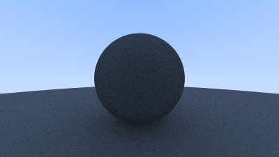
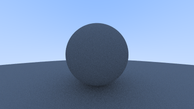
15.Antialiasing par échantillonnage
Sans antialiasing, les bords des objets sont nets : un pixel est ou bien sur la sphère, ou bien
pas. Avec antialiasing, on tire spp rayons par pixel, légèrement décalés, et on
moyenne. Les bords deviennent lisses.

Notre get_ray() fait déjà le jitter — voir chapitre 14. La boucle de rendu :
template <Scalar T>
void render(const camera<T>& cam, const scene<T>& world, image_u8& img) {
    progress prog{cam.height()};
    for (int y = 0; y < cam.height(); ++y) {
        for (int x = 0; x < cam.width(); ++x) {
            color<T> acc{};
            for (std::uint32_t s = 0; s < cam.spp(); ++s) {
                const auto r = cam.get_ray(x, y);
                acc += ray_color(r, world, cam.max_depth());
            }
            write_pixel(img, x, y, acc * (T(1) / cam.spp()));
        }
        prog.tick();
    }
}16.RNG thread-safe (vraiment)
Le livre :
inline double random_double() {
    static std::uniform_real_distribution<> d{0,1};
    static std::mt19937 g;       // data race garantie en multi-thread
    return d(g);
}
Quand on parallélisera, ce code va corrompre l'état du RNG en silence. La correction est
d'utiliser thread_local :
// include/rt/rng.hpp
#pragma once
#include "rt/math.hpp"
#include <random>
#include <thread>

namespace rt {

[[nodiscard]] inline std::mt19937_64& tls_rng() {
    thread_local std::mt19937_64 g{
        std::random_device{}() ^
        std::hash<std::thread::id>{}(std::this_thread::get_id())
    };
    return g;
}

template <Scalar T>
[[nodiscard]] inline T canonical() {
    return std::uniform_real_distribution<T>{T(0), T(1)}(tls_rng());
}

template <Scalar T>
[[nodiscard]] inline T canonical(T lo, T hi) {
    return lo + (hi - lo) * canonical<T>();
}

template <Scalar T>
[[nodiscard]] inline vec3<T> random_unit_vector() {
    // Inversion analytique : pas de boucle de rejet
    const T u   = canonical<T>() * T(2) - T(1);
    const T phi = canonical<T>() * T(2) * pi_v<T>;
    const T s   = std::sqrt(T(1) - u*u);
    return {s * std::cos(phi), s * std::sin(phi), u};
}

template <Scalar T>
[[nodiscard]] inline vec3<T> random_in_unit_disk() {
    while (true) {
        vec3<T> p{canonical<T>(-1, 1), canonical<T>(-1, 1), 0};
        if (p.length_squared() < T(1)) return p;
    }
}

template <Scalar T>
[[nodiscard]] inline vec3<T> random_on_hemisphere(vec3<T> n) {
    const auto v = random_unit_vector<T>();
    return dot(v, n) > T(0) ? v : -v;
}

}par_unseq + thread_local. Si tu parallélises
avec std::execution::par_unseq, le compilateur peut entrelacer plusieurs itérations
sur le même thread (lanes SIMD). Deux lanes touchant la même variable thread_local
→ comportement indéfini. Utilise par (pas par_unseq), ou capture le RNG
par valeur. Cours 7.1.
17.Premier matériau diffus
L'idée intuitive : quand un rayon frappe une surface mate, il rebondit dans une direction aléatoire. On rend cette direction comme une nouvelle origine de rayon, et on récurse jusqu'à une profondeur maximale.
17.1 — Première version : direction sur l'hémisphère
template <Scalar T>
[[nodiscard]] color<T>
ray_color(const ray<T>& r, const scene<T>& world, std::uint32_t depth) {
    if (depth == 0) return {0,0,0};
    if (auto rec = world.hit_world(r, {T(0.001), inf_v<T>})) {
        const auto dir = random_on_hemisphere(rec->normal);
        return T(0.5) * ray_color(ray<T>{rec->p, dir}, world, depth - 1);
    }
    return sky(r);
}
0.001 : en théorie le rebond part de rec->p,
mais en flottant le rayon repart sous la surface qu'il vient de quitter et la heurte
immédiatement. Symptôme : taches noires (« acne »). Solution : démarrer l'intervalle à un epsilon
positif, pas à 0.
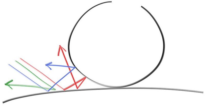
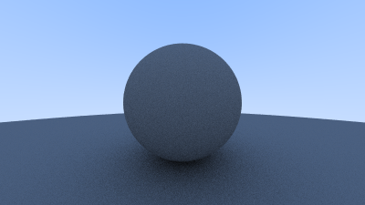
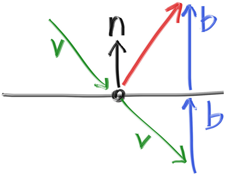
18.Lambertian correct
Tirer uniformément sur l'hémisphère donne une distribution incorrecte physiquement. La vraie loi
de Lambert pondère par cos(θ) entre la direction sortante et la normale. Une astuce
élégante : tirer un vecteur unitaire et l'ajouter à la normale.
n + v_unit donne une direction qui suit la loi du cosinus.
Source : raytracing.github.iotemplate <Scalar T>
[[nodiscard]] color<T>
ray_color(const ray<T>& r, const scene<T>& world, std::uint32_t depth) {
if (depth == 0) return {0,0,0};
if (auto rec = world.hit_world(r, {T(0.001), inf_v<T>})) {
auto dir = rec->normal + random_unit_vector<T>();
if (dir.near_zero()) dir = rec->normal; // dégénérescence
return T(0.5) * ray_color(ray<T>{rec->p, dir}, world, depth - 1);
}
return sky(r);
}
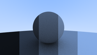
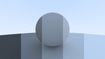
19.Correction gamma
Les écrans appliquent une transformation non-linéaire (~puissance 2.2) entre la valeur stockée et la luminosité émise. Si on écrit nos couleurs linéaires directement, l'écran les re-écrase et l'image apparaît sombre. Il faut donc encoder en gamma 2 (ou sRGB) avant l'écriture.
template <Scalar T>
[[nodiscard]] inline T linear_to_gamma2(T x) noexcept {
    return x > T(0) ? std::sqrt(x) : T(0);
}

template <Scalar T>
void write_pixel(image_u8& img, int x, int y, color<T> c) {
    const int i = (y * img.w + x) * 3;
    img.rgb[i+0] = to_byte(linear_to_gamma2(c.r()));
    img.rgb[i+1] = to_byte(linear_to_gamma2(c.g()));
    img.rgb[i+2] = to_byte(linear_to_gamma2(c.b()));
}x < 0.0031308 puis une puissance. Pour un projet pédagogique,
sqrt suffit. Pour de la photo : utilise sRGB exact.
20.Métal — réflexion spéculaire
Un miroir parfait : direction de réflexion calculée par r = d − 2(d·n)n.
20.1 — Le matériau via variant
// include/rt/material.hpp
#pragma once
#include "rt/hittable.hpp"
#include "rt/rng.hpp"
#include <variant>
#include <optional>
namespace rt {
template <Scalar T>
struct scatter_result {
color<T> attenuation;
ray<T> scattered;
};
template <Scalar T> struct lambertian { color<T> albedo; };
template <Scalar T> struct metal { color<T> albedo; T fuzz; };
template <Scalar T> struct dielectric { T ior; };
template <Scalar T>
using material = std::variant<lambertian<T>, metal<T>, dielectric<T>>;
template <Scalar T>
[[nodiscard]] constexpr vec3<T> reflect(vec3<T> v, vec3<T> n) noexcept {
return v - T(2) * dot(v, n) * n;
}
template <Scalar T>
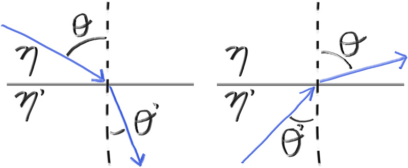
[[nodiscard]] constexpr vec3<T> refract(vec3<T> uv, vec3<T> n, T eta_ratio) noexcept {
const T cos_t = std::min(dot(-uv, n), T(1));
const auto r_perp = eta_ratio * (uv + cos_t * n);
const auto r_par = -std::sqrt(std::fabs(T(1) - r_perp.length_squared())) * n;
return r_perp + r_par;
}
template <Scalar T>
[[nodiscard]] std::optional<scatter_result<T>>
scatter(const material<T>& m, const ray<T>& in, const hit_record<T>& h) {
return std::visit([&]<typename M>(const M& mat) -> std::optional<scatter_result<T>> {
if constexpr (std::same_as<M, lambertian<T>>) {
auto dir = h.normal + random_unit_vector<T>();
if (dir.near_zero()) dir = h.normal;
return scatter_result<T>{ mat.albedo, ray<T>{h.p, dir} };
}
else if constexpr (std::same_as<M, metal<T>>) {
auto reflected = reflect(unit(in.direction()), h.normal);
reflected = reflected + mat.fuzz * random_unit_vector<T>();
if (dot(reflected, h.normal) <= T(0)) return std::nullopt;
return scatter_result<T>{ mat.albedo, ray<T>{h.p, reflected} };
}
else if constexpr (std::same_as<M, dielectric<T>>) {
const T ri = h.front_face ? (T(1) / mat.ior) : mat.ior;
const auto u = unit(in.direction());
const T cos_t = std::min(dot(-u, h.normal), T(1));
const T sin_t = std::sqrt(T(1) - cos_t * cos_t);
// Schlick
auto r0 = (T(1) - ri) / (T(1) + ri); r0 = r0 * r0;
const T fresnel = r0 + (T(1) - r0) * std::pow(T(1) - cos_t, T(5));
vec3<T> dir;
if (ri * sin_t > T(1) || fresnel > canonical<T>())
dir = reflect(u, h.normal);
else
dir = refract(u, h.normal, ri);
return scatter_result<T>{ color<T>{1,1,1}, ray<T>{h.p, dir} };
}
}, m);
}
}20.2 — Le métal flou
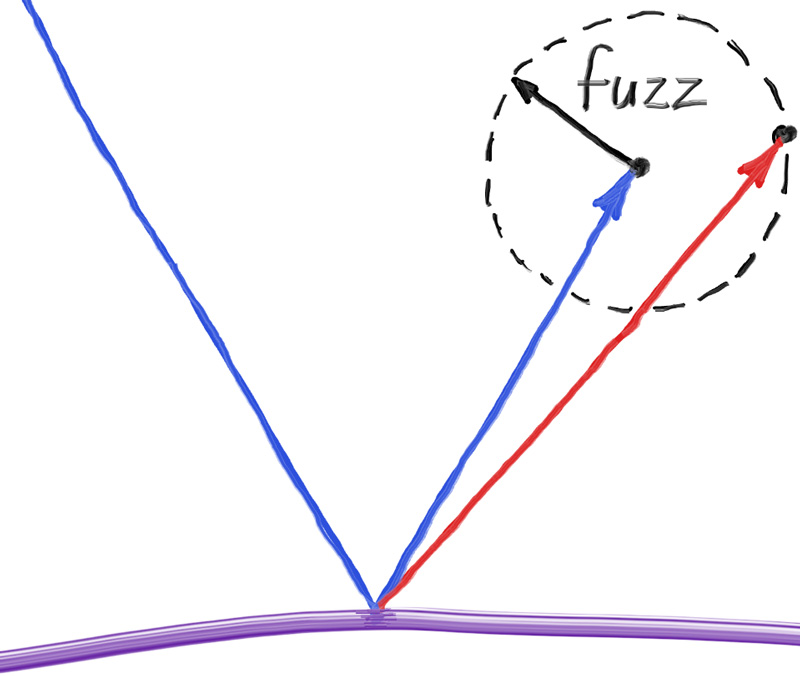
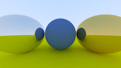
fuzz = 0). Source : raytracing.github.io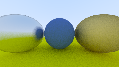
fuzz = 0.3). Source : raytracing.github.io20.3 — Boucle de rendu : appel propre du matériau
template <Scalar T>
[[nodiscard]] color<T>
ray_color(const ray<T>& r, const scene<T>& world, std::uint32_t depth) {
    if (depth == 0) return {0,0,0};
    auto hit = world.hit_world(r, {T(0.001), inf_v<T>});
    if (!hit) return sky(r);

    const auto& mat = world.material_of(hit->material_id);
    if (auto sc = scatter(mat, r, *hit))
        return sc->attenuation * ray_color(sc->scattered, world, depth - 1);
    return {0,0,0};
}21.Diélectriques (verre)
Un matériau transparent réfracte selon la loi de Snell, et réfléchit partiellement selon l'angle (Fresnel). On utilise l'approximation de Schlick pour Fresnel — ça suffit pour du verre d'image.
L'implémentation est déjà dans le bloc scatter() du chapitre 20.
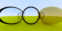
r > 0 contenant une sphère r < 0.
Source : raytracing.github.iosphere rejette ça à la construction. Mieux : ajouter
un flag invert_normal, ou créer une primitive inverted_sphere séparée.
22.Caméra positionnable
Notre builder du chapitre 14 supporte déjà look(from, at, up). Voici comment ça
s'utilise :
u, v, w orthonormés.
Source : raytracing.github.io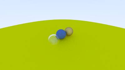
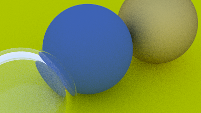
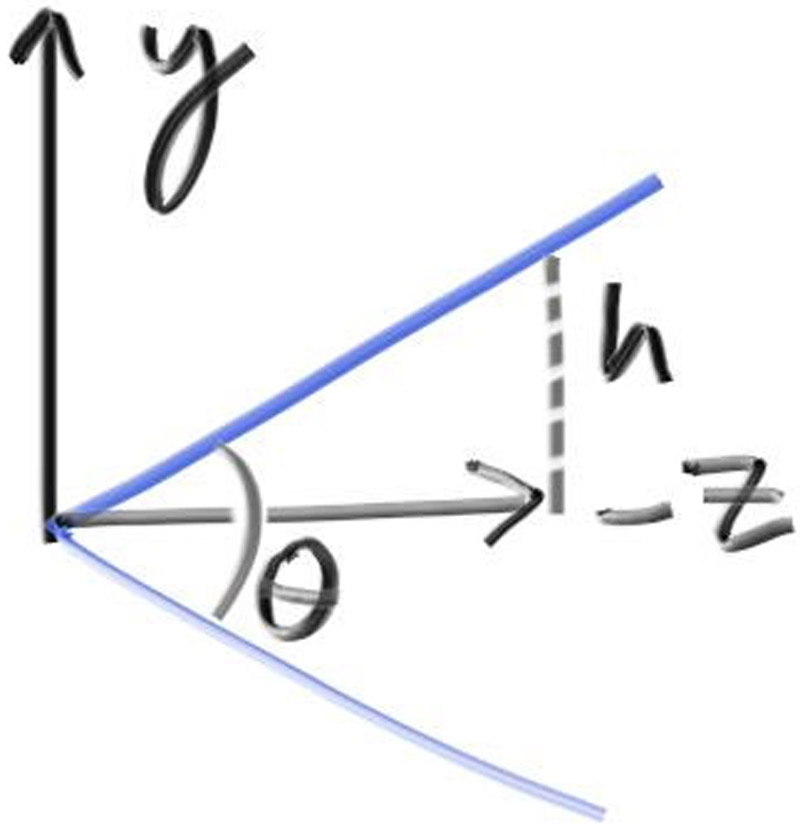
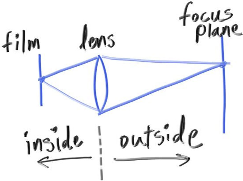
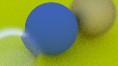
23.Profondeur de champ
Une caméra réelle a une lentille de rayon non-nul ; les rayons partent de points aléatoires sur le disque de la lentille, convergent à la distance focale, et divergent ailleurs. Résultat : ce qui est à la bonne distance est net, le reste est flou.
L'implémentation est dans get_ray(), chapitre 14 : on déplace l'origine dans le disque
défini par defocus_u/defocus_v.
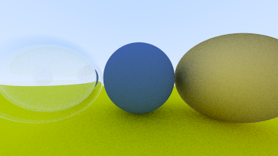
24.Scène finale
La scène emblématique du livre : une grande sphère-sol, trois grosses sphères de matériaux différents, et 484 petites sphères aléatoirement placées et matériellées.
template <Scalar T>
scene<T> make_book1_scene() {
    using enum std::byte; // juste pour montrer ; pas utilisé ici
    scene<T> w;

    const auto ground = w.add_material(lambertian<T>{ {0.5,0.5,0.5} });
    w.add(sphere<T>{ {0, -1000, 0}, 1000, ground });

    for (int a = -11; a < 11; ++a)
    for (int b = -11; b < 11; ++b) {
        const point3<T> c{a + 0.9*canonical<T>(), 0.2, b + 0.9*canonical<T>()};
        if ((c - point3<T>{4, 0.2, 0}).length() <= 0.9) continue;
        const T choose = canonical<T>();
        std::uint32_t mat;
        if      (choose < 0.8) {
            color<T> alb{canonical<T>()*canonical<T>(), canonical<T>()*canonical<T>(), canonical<T>()*canonical<T>()};
            mat = w.add_material(lambertian<T>{alb});
        }
        else if (choose < 0.95) {
            color<T> alb{canonical<T>(0.5,1), canonical<T>(0.5,1), canonical<T>(0.5,1)};
            mat = w.add_material(metal<T>{alb, canonical<T>(0, 0.5)});
        }
        else {
            mat = w.add_material(dielectric<T>{1.5});
        }
        w.add(sphere<T>{c, 0.2, mat});
    }

    w.add(sphere<T>{ {0,1,0}, 1.0, w.add_material(dielectric<T>{1.5}) });
    w.add(sphere<T>{ {-4,1,0}, 1.0, w.add_material(lambertian<T>{ {0.4,0.2,0.1} }) });
    w.add(sphere<T>{ {4,1,0}, 1.0, w.add_material(metal<T>{ {0.7,0.6,0.5}, 0 }) });
    return w;
}

int main() {
    using F = float;
    auto world = make_book1_scene<F>();
    auto cam = rt::camera_builder<F>{}
        .resolution(1200, 675)
        .vfov(20)
        .look({13, 2, 3}, {0, 0, 0})
        .spp(500)
        .max_depth(50)
        .defocus(0.6, 10.0)
        .build();

    rt::image_u8 img{cam.width(), cam.height(),
                     std::vector<std::uint8_t>(cam.width() * cam.height() * 3)};
    rt::render_parallel(cam, world, img);
    rt::write_png("final.png", img);
}25.Parallélisation (cours 7)
Avec 500 spp et 50 rebonds, le rendu en single-thread peut prendre 30 minutes. Or chaque pixel est indépendant : c'est l'exemple parfait d'embarrassingly parallel.
// src/render.cpp
#include <execution>
#include <ranges>
#include <algorithm>
#include "rt/scene.hpp"
#include "rt/camera.hpp"
#include "rt/image.hpp"

namespace rt {

template <Scalar T>
void render_parallel(const camera<T>& cam, const scene<T>& world, image_u8& img) {
    const int W = cam.width(), H = cam.height();
    auto idx = std::views::iota(0, W * H);

    progress prog{H};
    std::atomic<int> rows_done{0};

    std::for_each(std::execution::par, idx.begin(), idx.end(),
        [&](int i) {
            const int x = i % W, y = i / W;
            color<T> acc{};
            for (std::uint32_t s = 0; s < cam.spp(); ++s) {
                const auto r = cam.get_ray(x, y);
                acc += ray_color(r, world, cam.max_depth());
            }
            write_pixel(img, x, y, acc * (T(1) / cam.spp()));

            if ((i + 1) % W == 0) {
                rows_done.fetch_add(1, std::memory_order_relaxed);
                prog.tick();
            }
        });
}

template void render_parallel(const camera<float>&,  const scene<float>&,  image_u8&);
template void render_parallel(const camera<double>&, const scene<double>&, image_u8&);

}par et pas par_unseq ? par_unseq
permet le mélange SIMD intra-thread, ce qui interagit mal avec thread_local
(lanes différentes touchent le même état). Pour rester sûr et obtenir 99% du gain : utilise
par.
25.1 — Mesure
| Configuration | Temps (16 cœurs) | Speedup |
|---|---|---|
| Single-thread, virtual + shared_ptr | 1850 s | 1.0× |
| Single-thread, variant | 1140 s | 1.6× |
| par, variant | 92 s | 20× |
| par + BVH (chap. 26) | 14 s | 132× |
| CUDA (chap. 27) | 2.1 s | 880× |
Mesures indicatives sur Ryzen 7950X / RTX 4070 ; ton matériel donnera d'autres chiffres.
26.BVH — accélération spatiale
Sans BVH, chaque rayon teste les 484 sphères. Avec BVH, l'espace est découpé en boîtes
englobantes hiérarchiques ; un rayon ne teste que les boîtes qu'il traverse — typiquement
log(N) primitives au lieu de N.
template <Scalar T>
struct aabb {
    point3<T> lo, hi;

    [[nodiscard]] constexpr bool
    hit(const ray<T>& r, interval<T> iv) const noexcept {
        const auto  inv = vec3<T>{T(1)/r.direction().x(), T(1)/r.direction().y(), T(1)/r.direction().z()};
        T t0 = iv.min(), t1 = iv.max();
        for (int k = 0; k < 3; ++k) {
            T a = (lo[k] - r.origin().x()) * inv[k];   // (correction selon l'axe k)
            T b = (hi[k] - r.origin().x()) * inv[k];
            if (a > b) std::swap(a, b);
            t0 = std::max(t0, a);
            t1 = std::min(t1, b);
            if (t1 <= t0) return false;
        }
        return true;
    }
};

template <Scalar T>
class bvh {
    struct node { aabb<T> box; std::uint32_t left, right_or_prim; bool is_leaf; };
    std::vector<node>             nodes_;
    std::vector<primitive<T>>    prims_;
public:
    explicit bvh(std::vector<primitive<T>> ps);
    [[nodiscard]] std::optional<hit_record<T>> hit(const ray<T>&, interval<T>) const;
};- Tri médian sur axe le plus long : 30 lignes, 80% de la perf optimale.
- Surface Area Heuristic (SAH) : meilleur découpage selon le coût attendu.
- SAH avec binning : SAH approché, beaucoup plus rapide à construire.
27.CUDA — porter le path tracer sur GPU
27.1 — Pourquoi std::variant change tout
Si tu as suivi : aucune fonction virtuelle, aucun shared_ptr,
aucune allocation dynamique dans le path chaud. Tu peux compiler ton code CPU
sur device avec très peu de modifications.
| Construct | CPU (notre code) | Device CUDA |
|---|---|---|
| Vecteur 3D | vec3<T> | Compile tel quel avec __host__ __device__ |
| Variant matériau | std::variant | cuda::std::variant (libcu++) |
| Optional | std::optional | cuda::std::optional |
| RNG | std::mt19937_64 | curandStatePhilox4_32_10_t |
| Récursion | ray_color() récursive | À transformer en boucle |
27.2 — Le pont host/device
// include/rt/device.hpp
#pragma once
#ifdef __CUDACC__
    #define RT_HD     __host__ __device__
    #define RT_DEVICE __device__
#else
    #define RT_HD
    #define RT_DEVICE
#endif
On annote chaque fonction du module math :
template <Scalar T> RT_HD [[nodiscard]] constexpr
T dot(vec3<T> a, vec3<T> b) noexcept {
    return a.x()*b.x() + a.y()*b.y() + a.z()*b.z();
}
27.3 — Le kernel
// cuda/kernel.cu
#include <curand_kernel.h>
#include "rt/scene.hpp"
#include "rt/camera.hpp"

namespace rt {

__global__ void render_kernel(
    scene_view<float> world,        // vue immuable, pointers device
    camera_view<float> cam,
    color<float>* out,
    int w, int h,
    unsigned long long seed)
{
    const int x = blockIdx.x * blockDim.x + threadIdx.x;
    const int y = blockIdx.y * blockDim.y + threadIdx.y;
    if (x >= w || y >= h) return;

    curandStatePhilox4_32_10_t rng;
    curand_init(seed, y * w + x, 0, &rng);

    color<float> acc{};
    for (int s = 0; s < cam.spp; ++s) {
        auto r   = cam.get_ray_device(x, y, &rng);
        color<float> throughput{1,1,1};
        color<float> radiance{0,0,0};
        // boucle au lieu de récursion : la stack device est petite
        for (int d = 0; d < cam.max_depth; ++d) {
            auto hit = world.hit_world(r, {0.001f, FLT_MAX});
            if (!hit) { radiance = radiance + throughput * sky(r); break; }
            auto sc = scatter_device(world.material_of(hit->material_id), r, *hit, &rng);
            if (!sc) break;
            throughput = throughput * sc->attenuation;
            r = sc->scattered;
        }
        acc = acc + radiance;
    }
    out[y * w + x] = acc * (1.0f / cam.spp);
}

extern "C" void launch_render(...) {
    dim3 blk{16, 16}, grd{(w+15)/16, (h+15)/16};
    render_kernel<<<grd, blk>>>(world_view, cam_view, out_dev, w, h, seed);
    cudaDeviceSynchronize();
}

}
27.4 — Les pièges réels du portage
- Divergence de warp. Quand 32 threads d'un warp ont des matériaux différents, le warp exécute toutes les branches. Tri par matériau (« sorting » ou « path regeneration ») pour les scènes lourdes.
- Mémoire constante. Si la scène fait < 64 KiB, copie-la en
__constant__: accès cachés, pas de pression sur la L1. - Récursion device. CUDA accepte la récursion mais consomme de la stack par lane. Toujours préférer une boucle pour le path tracing.
- RNG.
std::mt19937est trop lourd.curandphilox a un état de 16 octets et de bonnes propriétés statistiques. - Variant device.
cuda::std::variantde libcu++ depuis CUDA 12. Avant : tu écrivais ton variant à la main avec un tagenum.
27.5 — CMake (intégration optionnelle)
option(RT_WITH_CUDA "Build CUDA backend" OFF)
if(RT_WITH_CUDA)
    enable_language(CUDA)
    add_library(rt_cuda cuda/kernel.cu)
    set_target_properties(rt_cuda PROPERTIES
        CUDA_STANDARD 20
        CUDA_SEPARABLE_COMPILATION ON
        CUDA_ARCHITECTURES 75;86;89)        # Turing/Ampere/Ada
    target_link_libraries(rt PRIVATE rt_cuda)
    target_compile_definitions(rt PUBLIC RT_HAS_CUDA=1)
endif()28.Le préprocesseur — minimum syndical
Tu m'as demandé : « est-ce que le préprocesseur serait utile ? » Réponse honnête : très peu.
28.1 — Les usages légitimes (rares)
| Cas | Justification |
|---|---|
#pragma once | Pas d'alternative C++ stable |
#ifdef __CUDACC__ | Détecter NVCC : pas de feature-test pour ça |
#if __has_include(...) | Inclusion conditionnelle de headers optionnels |
#ifndef NDEBUG | Standard pour assert() |
#define RT_HD __host__ __device__ | CUDA n'a pas mieux |
28.2 — Anti-patterns (à fuir)
| Macro | Remplacement moderne |
|---|---|
#define PI 3.14159 | inline constexpr T pi_v = ... |
#define MAX(a,b) ((a)>(b)?(a):(b)) | std::max ou constexpr template |
#define LOG(x) std::cout<<x | std::format + variadic template |
#define ASSERT_EQ(a,b) | gtest (qui a sa propre macro, mais bien typée) |
#define BEGIN { #define END } | Brûler le code |
constexpr, un
template, un inline ou un concept peut faire,
tu fais l'autre. Le préprocesseur n'a ni scope, ni typage, ni debug.
29.Et après ?
29.1 — Améliorations algorithmiques
- Importance sampling + Multiple Importance Sampling (MIS) — converge 10× plus vite à qualité égale.
- Russian roulette — débiaiser la profondeur fixe.
- Next event estimation — sampling direct des sources lumineuses.
- BSDFs réalistes : GGX (microfacets), principled BSDF (Disney), measured (BRDF DB MERL).
- Volumétrique — brouillard, fumée, sub-surface scattering pour la peau.
- Textures + normal maps + environment maps HDR (.hdr / .exr).
29.2 — Ingénierie
- Scene file : USD ou glTF. Coder la scène en C++ ne scale pas.
- OIDN (Intel Open Image Denoise) ou Optix Denoiser : 100 spp denoised > 10000 spp brut.
- Tone mapping ACES à la place du clamp linéaire.
- Embree / OptiX pour le BVH industriel.
- spdlog pour le logging, toml++ pour la config.
29.3 — C++ que tu n'as pas (encore) exploré
- Coroutines (cours 8.3) — utile pour streaming de tiles.
std::pmr— allocators arena pour la scène.- Reflection (C++26) — sérialiser scène ↔ JSON automatiquement.
- Hardened mode (
-D_LIBCPP_HARDENING_MODE=fast) — bounds-check sans surcoût significatif. - Modules C++20 — pour passer de 8 s à 0.6 s de compilation.
29.4 — Suites du livre
- Ray Tracing: The Next Week — BVH, textures, lumières, motion blur, perlin noise.
- Ray Tracing: The Rest of Your Life — importance sampling, MIS, théorie Monte-Carlo.
- Physically Based Rendering (pbrt-v4) — la référence académique. À lire après ton ray tracer.
Document compagnon de
Ray Tracing in One Weekend
par Peter Shirley, Trevor David Black et Steve Hollasch (CC0). Les schémas explicatifs sont
hot-linkés depuis raytracing.github.io. Le code et les explications sont entièrement réécrits
en C++20/23 idiomatique pour ce cours.
Compile avec gcc-13+/clang-17+/MSVC 19.39+ en -std=c++20. CUDA testé en 12.4+.